
Practical And Cost-effective Rendering - Character Skin
No matter what type or scale of your game, character rendering is an essential part of the project that is difficult to replace.
What’s interesting is that compared to everything in the world, we should be more familiar with our bodies. However, since the Renaissance, character drawing has always had a failure point, even from real-life models, both at the art and technical level. With the help of cutting-edge instrument scanning and extremely high texture accuracy, we still find it challenging to get rid of the troubles of the “Uncanny Valley” from time to time.
How can we have Cocos Creator help us make more easily believable character rendering? Cocos educator, raisins, shares his character rendering program.
Let’s start with the skin today.
Our Target Goal
We will write a subsurface scattering shader in the model, which expresses the skin material effect in character rendering. Cocos Creator already comes with the standard Metal/Roughness process PBR shader. We will add a new GLSL code on this basis so that all the PBR functions and features of the Metal/Roughness process can be used, and it also has subsurface scattering.
The most intuitive visual perception of subsurface scattering is that the object is illuminated from the inside out by its internal self-glow.
Our shader will be used with two new textures, Thickness and Curvature. These two terms must be familiar to students of graphic art, especially character art. At the same time, we will add the function of Fresnel reflection to give more flexible adjustment options based on the PBR reflection algorithm. Finally, we will give a Diffuse Profile function, the details of which will be described in detail later. At present, we only need to know that it is a function to adjust the color output with the value.
How to use this “Cocos Effect”?
Let’s Get Started Quickly
Cocos Effect is a format for Cocos Creator to store shaders. It is written in YAML. Cocos Effect integrates the parameters of the vertex shader, fragment shader, and editor into one file. It will be converted to different versions of OpenGL ES Shader, depending on the target platform. YAML only transmits data, and it does not contain logic. After all, the full name of YAML is “YAML Ain’t a Markup Language,” and it is the GLSL vertex and fragment shader that expresses the logic.
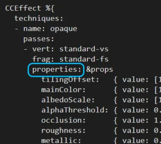
How to get the detailed information of Cocos Effect from the official document “Effect Syntax”(See the end of the post for the documentation links), take Cocos Creator’s built-in standard PBR shader as an example, we can refer to the following information to quickly start writing our own shader:
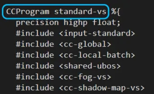
- All vertex shader codes need to be written in GLSL under the “CCProgram standard-vs” tab, and the built-in Shader parameters of Cocos Creator can also be used. The specific list can be obtained in “Common shader built-in Uniform.”
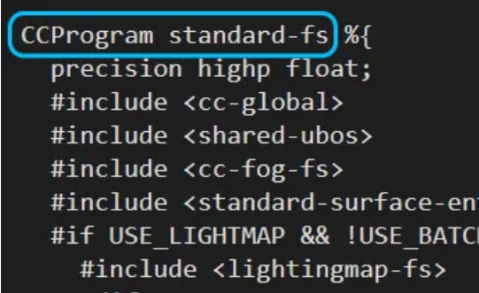
- Similarly, all fragment shader code needs to be written in GLSL under the “CCProgram standard-fs” tag;
- Custom parameters need to be declared under the “properties” label, and the variables declared under the “properties” label will appear in the edit panel in Cocos Creator;
- We need to declare a corresponding uniform for the newly declared parameters. This needs to be implemented under the “CCProgram shared-ubo” tag. The declared uniform can be accessed regardless of vertex shader or fragment shader;

- We can also declare custom functions, but remember: YAML does not contain logic. Therefore, the custom function should be placed in the vertex shader (“CCProgram standard-vs”) or the fragment shader (“CCProgram standard-fs”).
Laying out the theory
First of all, we need to answer a question: what kind of effect can make the skin more realistic?
We can find some references in real life:
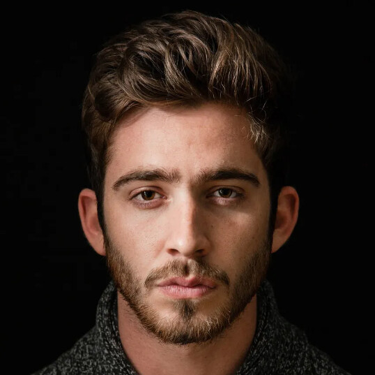
Looking at the picture above, the first thing you may notice is that his ears are redder. In addition, the steeper the structure and the harder the lines, the red appears more intense. In addition, a red-colored band can also be seen at the junction of light and dark on the bridge of his nose.
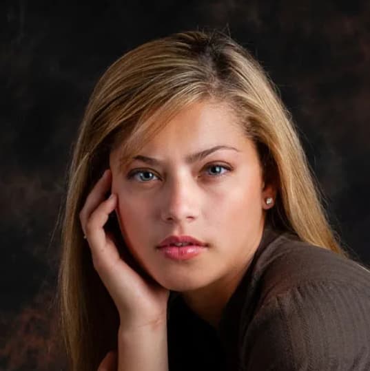
In the above picture, we can also observe the red color band on the border of light and dark on the bridge of the nose. The line of her nose bridge is not particularly steep, so the color band seems to be wider than the previous example.

In this example, we can also observe the red clusters, but on her face, red clusters at the nose and nose.
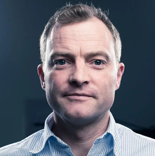
In this example, we can see a large area of pink clusters at the junction of light and dark on his cheeks (as for why it is pink, it is because this photo was mixed with cool colors in the post-grading). And this pink can also be seen in the sharp part of his nose.
Taken together, we seem to be able to observe certain patterns:
- In the part of the human skin where the light and dark lines intersect, there will be red clusters.
- The red color will be more evident and vivid in the parts where the face structure is steep and the lines are sharp.
- The ears, tip of the nose, and wings of the nose are common places where red color gathers.
So, why does this phenomenon occur? Where do these reds come from exactly?

We know that when the rays of light from a medium A goes into another medium B, part of the light is reflected or absorbed by medium B. Other rays enter medium B, and after repeated reflection and refraction, they finally are refracted back into medium A. These light rays are captured by the human eye. The human eye captures the light and observes the color of medium B. Although these rays are, in principle, reflected rays (Specular), they are actually scattered (Diffuse) qualities, so they are called Diffuse Reflectance rays.
You have probably noticed that when the diffusely reflected light passes through various processes in medium B and re-injects into medium A, it is already a certain distance from the point of incidence that originally entered medium B. For most materials, this distance is minimal and can be ignored entirely, so we can understand that the diffuse reflection light is emitted from the original incident point.
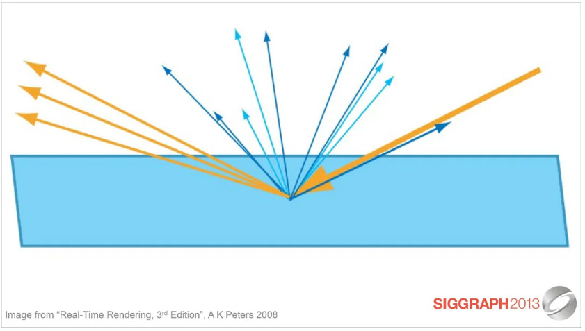
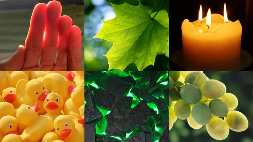
However, for a small number of materials, this distance cannot be ignored. When light enters this kind of material, it will show a characteristic of light transmission, as if the object has its own light source inside, illuminating the object from the inside. Many organic materials in nature exhibit this characteristic, such as beeswax, leaves, fruits, vegetables, and of course, human skin.
This special scattering characteristic is called Sub-surface Scattering.
The principle seems quite simple, but how should we achieve it?
In the history of computer graphics, we can find various techniques for expressing subsurface scattering. One of the earlier examples comes from the movie “The Matrix.” Special effects staff found that they can simply blur the Diffuse texture of the skin and superimpose it on the original texture to effectively reduce the texture’s artificial look and create the effect of light scattering under the epidermis.
As for the red accumulation on the light-dark boundary line, you probably have thought that you can easily use the “N·L” method to calculate the position of the light-dark boundary line through the light direction and the surface normal of the object, and then superimpose it with a color. This method is also known as the Wrap Lighting method and is widely used in the classic game “Half-life 2”.
And “N-L” is very similar to the “N-V” method. You can get through the camera direction and the object surface normal to the camera viewing angle of the part of the object, which can help us easily obtain the Fresnel reflection effect.
Speaking on this, our goal has been relatively straightforward:
- We need a blur to achieve the diffuse reflection effect of the Diffuse texture.
- We need a Thickness map and a Curvature map to help us identify those parts of the object prone to subsurface scattering.
- We need a Fresnel reflection effect, which will help us realize the Specular part of the skin.
- Finally, we need a Diffuse Profile, which will help us determine the intensity and color of the subsurface scattering.
Achieve blur effect
How to achieve the blur effect? The logic behind it is actually very simple: we only need to offset the UV of the IMAGEthat needs to be blurred a little distance in each direction, add all the offset results, and find an average value:
vec3 boxBlur( sampler2D diffuseMap,  float  blurAmt ){
 vec2 uv01 = vec2(v_uv.x-blurAmt * 0.01, v_uv.y-blurAmt * 0.01);
     vec2 uv02 = vec2(v_uv.x + blurAmt * 0.01, v_uv.y-blurAmt * 0.01);
     vec2 uv03 = vec2(v_uv.x + blurAmt * 0.01, v_uv.y + blurAmt * 0.01);
     vec2 uv04 = vec2(v_uv.x-blurAmt * 0.01, v_uv.y + blurAmt * 0.01);
     vec3 blurredDiffuse = (SRGBToLinear(texture(diffuseMap, uv01).rgb) + SRGBToLinear(texture(diffuseMap, uv02).rgb) + SRGBToLinear(texture(diffuseMap, uv03).rgb) + SRGBToLinear(texture(diffuseMap, uv04)).rgb) / 4.0;
 return  blurredDiffuse;
}
In the above sample code, “v_uv” is the UV data passed by the Vertex Shader. We write our Shader based on the built-in PBR shader of Cocos Creator, so there are a lot of preparations already done. We can just use it directly. “SRGBToLinear” is a built-in function of Cocos Creator, which converts color data in sRGB space into linear space. In the PBR process, all color calculations need to be performed in linear space.
Of course, just calculate the average value once, and the final effect may not be particularly good. You can also use the same method to loop 2-3 times to get a more soothing effect:
vec3 blurPass = vec3( 0.0, 0.0, 0.0 );
for (  float  i = 1.0; i <4.0; i++ ){
 blurPass += boxBlur(diffuseMap, blurAmt * i);
}
blurPass = blurPass / 3.0;
This single-handed blurring method is called Box Blur. Its characteristic is that all pixels are treated equally and are processed at the same level of blur. Although concise and efficient, it is not necessarily what we want visually.
If you have used the Adobe series of IMAGEprocessing tools, you must be familiar with the most commonly used blur tool Gaussian Blur. The logic of Gaussian blur is the same as that of a square blur. The difference is that the larger the pixel offset, the higher the degree of blur, and vice versa. The weight of the blur degree is arranged in a normal distribution. In this way, the result we get is low in the middle and high in the surroundings, and it shows a natural attenuation effect from the middle to the surroundings.
It seems like it’s too much trouble to implement a normal distribution function from scratch with code. Fortunately, we only need a few normally distributed values as our fuzzy weights, which can be directly substituted into our square fuzzy function. There are many normal distribution value generators available online.
vec3 gaussianBlur( sampler2D diffuseMap,  float  blurAmt) {
 float  gOffset[5];
 gOffset[0] = 0.0;
 gOffset[1] = 1.0;
 gOffset[2] = 2.0;
 gOffset[3] = 3.0;
 gOffset[4] = 4.0 ;

 float  gWeight[5];
 gWeight[0] = 0.2270270270;
 gWeight[1] = 0.1945945946;
 gWeight[2] = 0.1216216216;
 gWeight[3] = 0.0540540541;
 gWeight[4] = 0.0162162162;

 vec3 baseDiffuse = SRGBToLinear(texture(diffuseMap , v_uv).rgb);
 for (int i = 0; i <5; i++ ){
  baseDiffuse += SRGBToLinear(texture(diffuseMap, v_uv + vec2(gOffset[i] * 0.01 * blurAmt, 0.0)).rgb) * gWeight[i];
  baseDiffuse += SRGBToLinear(texture(diffuseMap, v_uv-vec2(gOffset[i] * 0.01 * blurAmt, 0.0)).rgb) * gWeight[i];
  baseDiffuse += SRGBToLinear(texture(diffuseMap, v_uv + vec2(0.0, gOffset) [i] * 0.01 * blurAmt)).rgb) * gWeight[i];
  baseDiffuse += SRGBToLinear(texture(diffuseMap, v_uv-vec2(0.0, gOffset[i] * 0.01 * blurAmt)).rgb) * gWeight[i ];
 }
   return  baseDiffuse / 5.0;
}
Explore Diffuse Profile
Let’s go back to the red cluster on the borderline between light and dark that we observed earlier. We thought we could use “N·L” + color superposition to achieve this effect, but here is a question: Is the red here a constant red?
Let’s look at an experiment: a sphere exhibiting subsurface scattering, illuminated by a single light source. The light source’s position and intensity remain unchanged, the sphere’s size is enlarged and reduced, and the change of the scattering color of the subsurface can be observed.
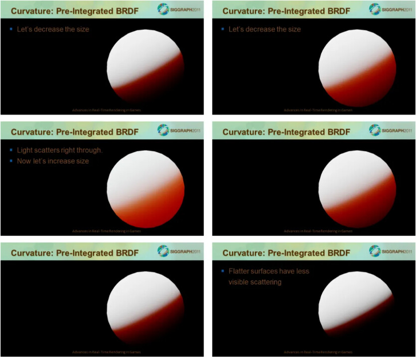
The result is slightly unexpected: when the sphere is very large and very small, the scattering color is darker, almost pure black. As the sphere zooms close to a range between the maximum and the minimum, the scattered color gradually becomes brighter and vivid until it reaches a peak.
This seems to tell us: the color change of the subsurface scattering also follows a bell-shaped curve (normal distribution curve), reaching a peak at a certain critical point and decreasing to both sides.
So, what determines this critical point? It depends on how we understand the change in the size of the sphere in the experiment.
First of all, when the position of the light source does not change, the size of the sphere changes, which means that the distance that the light travels on the surface of the sphere changes. That is to say, the distance that the light travels is one of the factors.
In addition, a sphere with a larger radius can be seen as having a larger curvature on its surface and vice versa. A sphere with an infinitely small radius also has an infinitely small curvature of its surface and can be seen as a flat surface. That is to say, the curvature of the object’s surface, i.e., the degree of curvature, is also a factor. This also fits with the conclusion we obtained earlier in the observation of the reference diagram.
The theory is beautiful, but how do we achieve it?
Fortunately, we already have skin subsurface scattering data based on real-world observations for us to use:
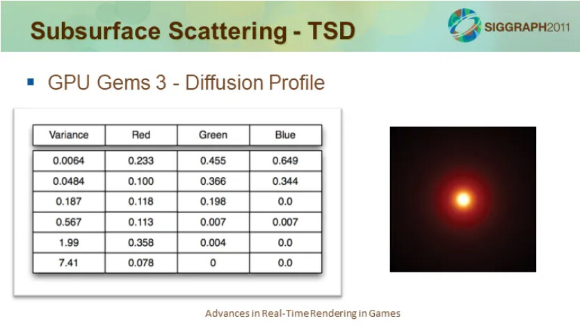
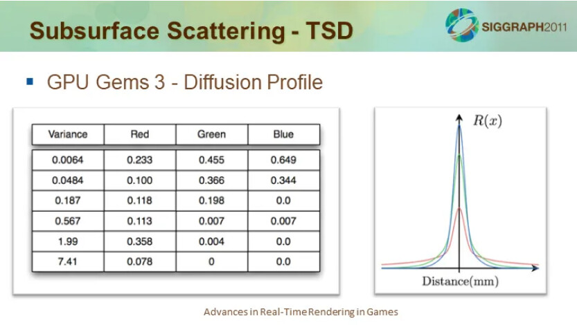
This table looks a bit unclear. To put it simply: the red on the skin we observe is actually the result of different sections of the skin being scattered with different colors and intensity curves, and then superimposed. This table lists six layers of different colors and curves. The scattering intensities of all cross-sections are arranged in a normal distribution so that we can see the naturally attenuated blooming in the right image.
Now that the data has been given to us, we can calculate the scattering intensity according to the normal distribution formula and then superimpose it with the color. The final output of the scattering is solved.
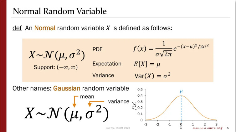
The above figure is the normal distribution (Gaussian distribution) formula. Simply put: μ is the median, which is the peak value of the scattering color in our calculations. We know the distance traveled by the light and the curvature of the surface of the object. Currently, it can be 0. σ^2 is the variance, which determines the steepness of the bell curve, and this value has been provided for us. From this, we can directly bring in the formula:
#define M_PI 3.1415926535897932384626433832795
 vec3 Profile(  float  dis ){
 return   vec3(0.233, 0.455, 0.649) * 1.0 / (abs(sqrt(0.0064)) * abs(sqrt(2.0 * M_PI))) * exp(-dis * dis / (2.0 * 0.0064)) +
  vec3(0.1, 0.366, 0.344) * 1.0 / (abs(sqrt(0.0484)) * abs(sqrt(2.0 * M_PI))) * exp(-dis * dis / (2.0 * 0.0484) ) +
  vec3(0.118, 0.198, 0.0) * 1.0 / (abs(sqrt(0.187)) * abs(sqrt(2.0 * M_PI))) * exp(-dis * dis / (2.0 * 0.187)) +
  vec3(0.113 , 0.007, 0.007) * 1.0 / (abs(sqrt(0.567)) * abs(sqrt(2.0 * M_PI))) * exp(-dis * dis / (2.0 * 0.567)) +
  vec3(0.358, 0.004, 0.0) * 1.0 / (abs(sqrt(1.99)) * abs(sqrt(2.0 * M_PI))) * exp(-dis * dis / (2.0 * 1.99)) +
  vec3(0.078, 0.0, 0.0) * 1.0 / (abs(sqrt(7.41)) * abs(sqrt(2.0 * M_PI))) * exp(-dis * dis / (2.0 * 7.41));
}
So far, we have obtained the blur to achieve the Diffuse scattering effect and the Diffuse Profile that solves the color and intensity of the subsurface scattering. The question now is: Where should the subsurface scattering appear?
Here we need to introduce two textures: Thickness and Curvature. Thickness calculates the thickness of an object by emitting rays in the opposite direction of the normal, and Curvature represents the curvature of the object’s surface. We don’t need to consider how to calculate and generate these two images in the engine because we can render them offline in third-party software, such as Substance Painter.
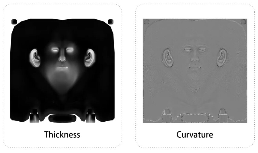
After getting the baked texture, we put Curvature aside and deal with Thickness first.
vec4 bDepth = gaussianBlur(thicknessMap, 0.0);
float  deltaDepth = abs(SRGBToLinear(texture(thicknessMap, v_uv).rgb).x-bDepth.x);
We first use the Gaussian blur to process Thickness and then subtract the blurred Thickness texture from the original texture. Recall the principle of Gaussian blur. The result we get is: after blurring, the pixels with more minor deviations are subtracted, leaving behind the pixels with more significant deviations. These delta values can be used as a mask for our subsurface scattering.
The one we still lack is the Fresnel reflection. As mentioned above, we can use the “N·V” method to achieve this effect.
vec4 v_normal_cam = normalize(cc_matView * vec4(v_normal, 0.0));
float  NVdot = dot(vec3(0.0, 0.0, 1.0), normalize(v_normal_cam).xyz);
In the above sample code, “cc_matView” is a parameter of Cocos Creator, and what returns is the attempt matrix. “V_normal” is the normal data passed from the Vertex Shader.
All the components are basically ready. The following is linking them up.
Finishing the shader
For the diffuse reflection effect, use our blur to process the Diffuse texture and overlay it on the Albedo channel.
vec4 bDiffuse = gaussianBlur(diffuseMap, blurAmt);
s.albedo += bDiffuse;
For the effect of Fresnel reflection, use the weight calculated by our “N·V,” multiply it by a custom parameter, and add it to the roughness channel.
pbr.y += NVdot * roughnessGain;
s.roughness = clamp(pbr.y, 0.04, 1.0);
For the diffuse color, we’ve got the Diffuse Profile function. The question is: What parameters to bring into this function?
We already know that the distance the light travels and the curvature of the object’s surface are factors that affect the scattering of the subsurface. The distance traveled by light seems more challenging to control. Still, we at least know that the front-to-back relationship of the object itself is also included in the distance traveled by the light, so it is logical to substitute the vertex position data (v_position).
As for the curvature of the surface of an object, we don’t know the direct numerical relationship between curvature and subsurface scattering, but we know through observation experiments that the relationship between curvature and subsurface scattering intensity is roughly linear. So let’s take the curvature (provided by the Curvature map), treat it as a general numerical weight, and adjust it with our custom weight.
In addition to the output of Diffuse Profile, we can also use the built-in cc_mainLitColor parameter of Cocos Creator to add the influence of the color and intensity of the light source to the scattering.
Finally, the object’s diffuse color is superimposed on the color output to establish the color and intensity of the subsurface scattering.
vec3 curvatureMap = SRGBToLinear(texture(curvatureMap, v_uv).rgb);
vec3 sssColor = Profile(length(v_position) * curvatureMap.x) *
                cc_mainLitColor.rgb *
                cc_mainLitColor.w *
                s.albedo.rgb;
However, the question arises again: From which channel should the subsurface scattering be our output?
Cocos Creator follows the standard PBR Metal/Roughness process. There is no Translucency channel in the Pipeline by default, but this will not affect us much: we can use the Emissive channel to achieve the same effect.
The next question is: Where should subsurface scattering occur?
We know that the cause of subsurface scattering is the internal luminescence phenomenon caused by the reflection and refraction of incident light inside the object, so our first step is to calculate “N·L.” Using the Thickness Δ value we have obtained, we can get a clear The face is 0, and the dark face is the thickness mask. This is also in line with the principle of subsurface scattering: light enters from the bright surface so that we can observe the phenomenon of subsurface scattering from the dark surface.
Finally, use the mask to superimpose the subsurface scattering color on the dark surface, and our effect is already out.
float  sssMask = mix(deltaDepth, 0.0, NLdot);
vec3 sssGain = mix(vec3(0.0, 0.0, 0.0), sssColor, sssMask);
s.emissive += sssGain;
Subsurface scattering is indeed an enduring topic. There is no doubt that many areas can be corrected, improved, and further explored in our results today. I hope you read this, have inspired some whimsical ideas, and started making your own Cocos Creator shader.
In the next chapter, we will look at how to render realistic character hair in Cocos Creator.